PAOC Spotlights
Quantifying Parameter and Structural Uncertainty in Climate Modeling

Read this at CliMA
Robustly predicting Earth’s climate is one of the most complex challenges facing the scientific community today. By leveraging recent advances in the computational and data sciences, researchers at CliMA are developing new methods for calibrating climate models and quantifying their uncertainties.
In today’s climate models, the primary source of uncertainty are approximations of processes that cannot be explicitly resolved, such as turbulence in atmosphere and oceans and the convection sustaining clouds. These approximations, known as parameterization schemes, are a set of physical equations that, given some environmental conditions (such as wind and temperature) supplied by the climate model, predict the approximate effect of each unresolved process. In addition to the environmental conditions, the schemes also require parameters, which are often fixed to values based on a limited number of empirical studies. Two main types of uncertainty can arise, one from insufficient knowledge of the parameter values fed into the scheme (parameter uncertainty), and the other from the coarseness/approximations of the equations in the scheme (structural uncertainty).
The chaotic nature of the atmospheric equations can lead to a sensitive and complex dependence of climate on the parameters, so that in some cases (most notably within convection parameterizations), a small misestimation of a parameter can lead to a dramatically different representation of the approximated process. Fixing parameters to a single value everywhere when making predictions leads to uncertainties, which remain hidden and unquantified. In light of that, instead of using one specific value for a parameter, our researchers apply statistical methodologies from the area of Bayesian inverse problems, where the solution for the parameterization is found as a distribution over many possible parameters. This distribution has a structure that is refined by data from satellites and targeted highly resolved explicit simulations of the physical process in question. As more data are collected (eventually this will include automated on-the-fly integration of high-resolution simulations), the distribution gradually becomes tighter. By feeding our model with the quantitative distribution of “possible parameters,” we will be able to obtain a corresponding range of “possible predictions,” and make reliable probabilistic inferences for climate impacts at each location and time, similarly to what is currently done for weather forecasts.

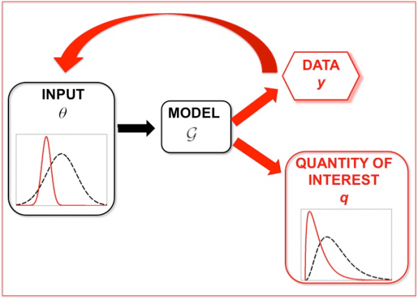
Figure 1: The uncertainty quantification pipeline. A data-uninformed distribution of inputs (black dashed) leads to a corresponding distribution of a quantity of interest (black dashed). Due to the inclusion of data, with a learning loop, we refine the prior to a data-consistent “posterior” distribution of inputs (solid red), leading to prediction of the quantity of interest with more meaningful distribution (solid red).
Because running climate models with different parameter settings is computationally costly, our data assimilation and machine learning team at CliMA has developed a modular strategy that is computationally very efficient. First, a highly-parallelizable ensemble-based scheme is used to locate the approximate region of realistic parameter values. A state-of-the-art machine learning technique then develops a surrogate model, trained on information collected from the ensemble simulations to accurately reproduce data over this region of realistic parameters.The surrogate allows us to obtain data for new parameter values at a negligible cost, allowing us to make use of algorithms for refining the parameter distribution with satellite or simulation data previously out of reach due to the computational expense. When one needs to make a prediction of the climate, these refined distributions are fed back into the real climate model to produce a refined distribution of predictions to assess the climate impacts of interest.

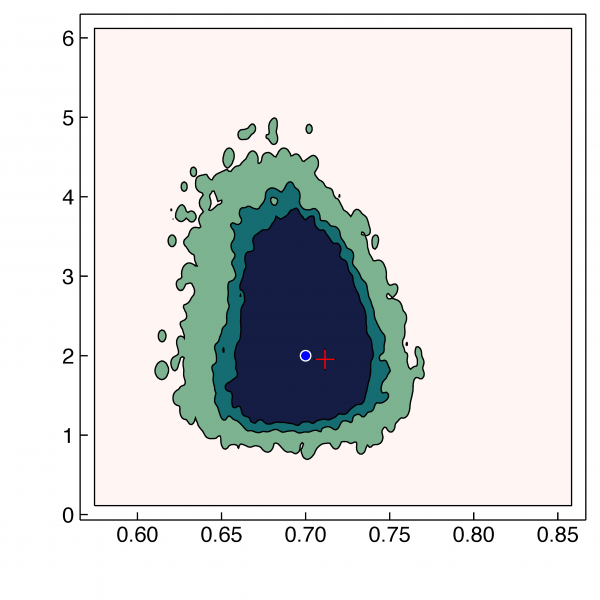
Figure 2: The posterior distribution in a climate application from learning two convective parameters with noisy data (the contours contain 50%,75%, and 99% of the distribution respectively). The prior parameters – not plotted – have a range of [0,1] and [0,60]. The true parameters (blue dot) that created the synthetic data used here and “optimal parameters” (red plus) are plotted. This is the 2D analogue of the input (solid red) curve in Figure 1.
This technique, referred to as the Calibrate, Emulate, Sample method is detailed in a recent publication. The methodology’s name reflects the three steps described above. It is an inexpensive and flexible solution, applicable in many settings. We demonstrate its success for estimating parameter uncertainty of convection parameters in a very idealized climate model in a recent submission, Calibration and Uncertainty Quantification of Convective Parameters in an Idealized GCM.

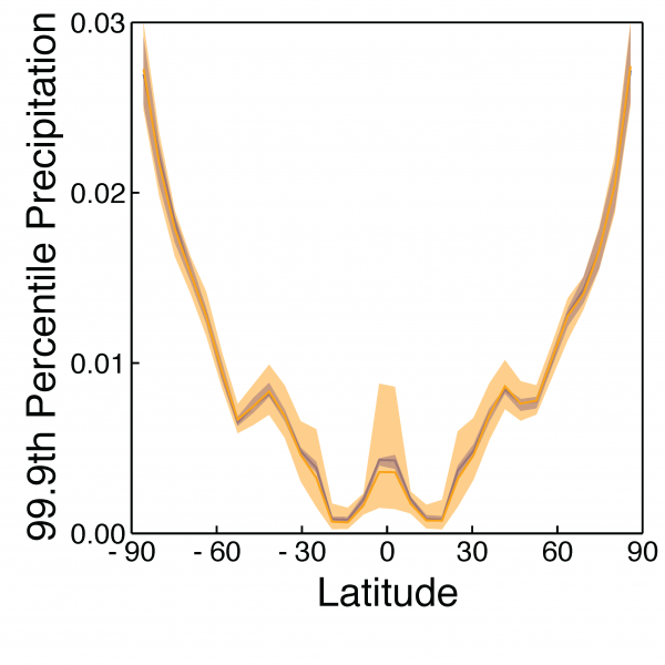
Figure 3: A prediction of a quantity of interest in a global warming experiment. What is plotted is the frequency with which what is a 1-in-1000 day extreme precipitation event in a control climate occurs in a warmed climate. For example, in polar regions, a 1-in-1000 day extreme precipitation even in the control climate becomes a 1-in-30 day event in the warm climate. Predictions of the quantity are shown with fixed parameters (purple) and with quantified parameter uncertainty from the distribution in Figure 2 (orange). The uncertainty bounds give robustness to the significance of this result across the range of data-consistent parameters, and shows where predictions are particularly uncertain (e.g., in the tropics).
The structural uncertainty comes from the inability of the climate model to resolve every detail of Earth’s climate through numerical simulations, and from the inability of parameterizations to represent small-scale processes entirely correctly. The approximations and limitations of representing the physics of these subgrid-scale processes causes uncertainties in the structure of the model itself, known as structural uncertainty. To address structural uncertainty, our researchers have made two assumptions: that the structural uncertainty can be approximated by a set of basis functions and a stochastic process, and that nature always favors simplicity. The problem of quantifying structural uncertainty is then converted into learning a sparse solution of unknown coefficients for the basis functions and the stochastic process. The specific choices of basis functions can be guided by domain knowledge, where information for data-driven modeling and physics merge.
In our uncertainty quantification framework, uncertainty information a posteriori can also be used to make structural improvements to the climate model and can even guide the development of new parameterizations. To develop parameterizations, our team runs high-fidelity numerical simulations of small-scale processes and adjusts unknown parameters in the parameterization to match known physics. The estimation of the uncertainty of the unknown parameters is critical, and the gap between the small-scale processes and the large-scale processes is bridged through a consistent Bayesian framework. To illustrate the methodology of Bayesian learning, CliMA researchers at MIT used a typical Ocean parameterization (the K-Profile Parameterization) to show that this parameterization exhibits a systematic bias, and then showed how to adjust the parameterization to account for the bias in the scenarios examined.
By developing and implementing these new computational methodologies in our climate models, we are making significant steps in quantifying uncertainty in climate models, and in using this information to guide improvements to climate models; this marks vital progress in working on our goal of reducing uncertainty in climate models.
Story Image: Earth at night, focusing on the Southeastern United States, taken from aboard the International Space Station, orbiting 250 miles above the planet. Credit: NASA/Mark Vande Hei